Visualizing Similarity with Distance

Copyright (c) Aleks Jakulin, 2004. [e-mail] (remove unnecessary dashes and spaces from the e-mail address to respond)

We have to distinguish similarity, which is in our case defined through a statistical model, and distance defined geometrically. We can employ various algorithms with the purpose of presenting the statistical similarities in the form of distances, clarifying the structure in data.

The colors are derived from bloc memberships in the latent variable model. The perceptual similarity of color marks the similarity as it arises in the latent variable model.

Principal Component Analysis:

This is the most frequently used method of analyzing high-dimensional data. Each senator can be understood as a variable. Should we consider each of the senators and the outcome, we would have a 101-dimensional space. Fortunately, because of correlations and structure in the senators' votes, we can project the data to a lower-dimensional space which nevertheless captures most of the variation. The two dimensions can be seen as representing axes of variation. The horizontal one separates Democrats from Republicans, while the vertical one is a bit more difficult to characterize.

However, it is important to assume how to represent situations when a senator did not vote. Of course one can obtain the maximum likelihood values (what is the most likely vote for the senator), but this carries certain assumptions. On the other hand, we can represent each senator with two dimensions (201 dimensions overall), but we are not particularly interested in modeling when someone would or would not vote. The following diagrams examine the arrangement of senators as obtained by PCA, but depending on the assumption of how to interpret "Not Voting". Depending on the imputation method, two dimensions captured 70.0% - 77.2% of total variation, as assessed by the R^2 statistic.

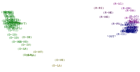Imputation by Absence

We assume that when a senator did not vote, we are best off guessing that he or she would vote like those senators that usually vote similarly as our senator. We "interpolate" the missing values. This corresponds to a situation when a senator was prevented from voting, or would want to vote but could not.

The outcome is near the Republican aggregation of points.

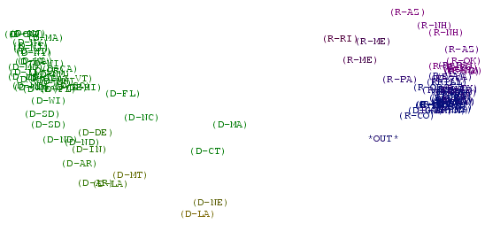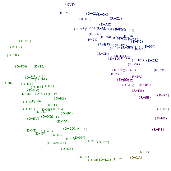
Imputation by Stratagem

By stratagem we assume that the senator did not vote consciously. This corresponds to letting the majority decide in his name.

We observe that those senators that did not vote often (e.g., Kerry (D-MA) and Lieberman (D-CT) ) end up in the space between both parties.

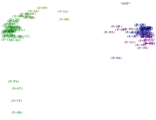Imputation by Submission

By submission we mean that a senator did not vote consciously because he or she could not change the outcome of the vote. Therefore, the true vote is understood to be the opposite of the eventual outcome.

The senators that did not vote often (Kerry (D-MA), Lieberman (D-CT), Edwards (D-NC) and Graham (D-FL) ) end up in a separate branch.

Multi-Dimensional Scaling with Rajski's distance:

We represent each senator as a point in space, and compute the distance between each of them using Rajski's distance. We then try to place the positions of senators so that the Euclidean distance is as close to the similarity as possible. This problem is referred to as multi-dimensional scaling.

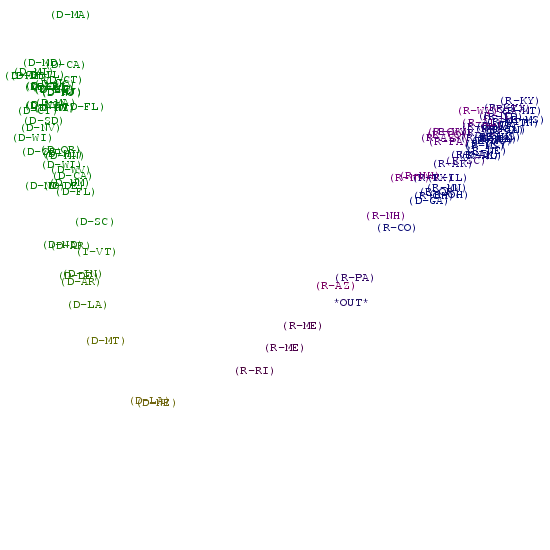Torgerson's MDS procedure

This is a very fast procedure based on the Singular Value Decomposition algorithm. This procedure is usually used as the first approximation before applying SMACOF.

SMACOF MDS procedure

This is an iterative procedure for matching similarities with Euclidean distances. The points are moved iteratively in a hypothetical space in order to best capture the Rajski's distance between each pair of senators.

Binary PCA:

De Leeuw's "binary PCA" attempts to explain the votes with a simpler statistical model. Each senator is represented as a point, and each issue is represented as a line that separates those who voted for from those who voted against a particular bill. The separation is not perfect, but the algorithm attempts to move the ideal points around so that the error that these lines make is as low as possible. Similarity between senators is not considered explicitly, but indirectly through the representation of votes. This model is one of several in the family of "classification" models (because the objective criterion is how well we can classify the votes). These models are most similar to those typically used in political science for interpreting the roll call data. It must be noted, however, that the modern models in political science are based on assumptions about decision-making and utility: the models we examine do not concern themselves with decision-making, solely with representation.

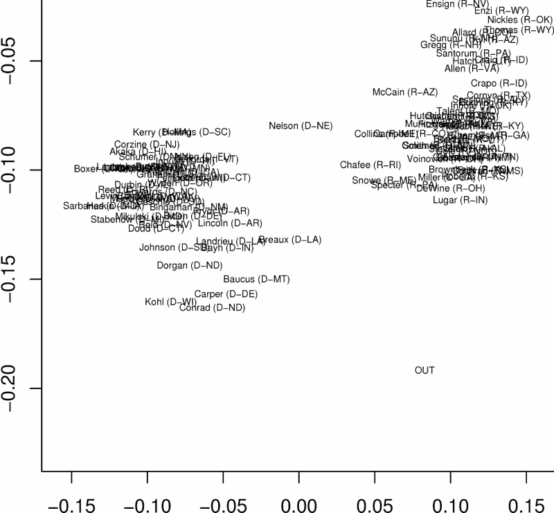Ideal Points

Each senator is placed somewhere in the 2D space. Although the similarity between senators is not a criterion in the optimization, we observe a very similar structure of groups as with the analyses above.

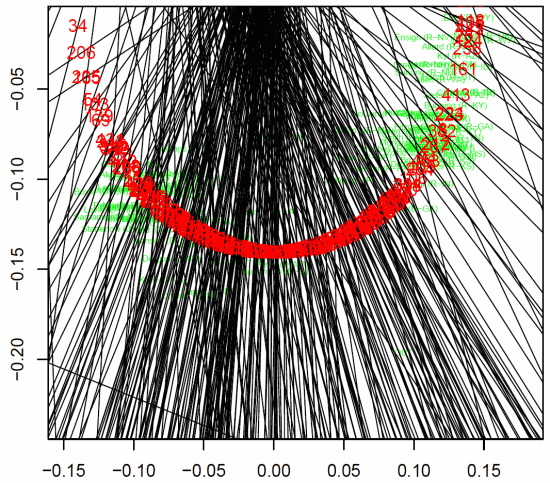Votes

Each vote can be represented as a line that separates the senators who voted for and against the issue. The objective criterion is to minimize the number of misclassifications.

We can see that most of the votes split the Democrats, but very few votes split the Republicans. In a few cases, the vote was unanimous: note the lines around the edges of the diagram.

The issue of John Kerry:

National Journal claimed that Kerry is an extreme liberal. This was disputed by many, including Kerry himself. Poole claims that Kerry is liberal but not extreme [link, link], Clinton, Jackman & Rivers say that it's hard to say due to his absenteeism but also that Kerry is not extreme [PDF link].

However, one should interpret "Not Voting" as letting the majority vote for you. Since the majority is Republican, the fact that Kerry often did not vote means that he is effectively the most central of all Democrats, based on all the votes cast in 2003.